palmerpenguins %>%
  ggplot(aes(x = species, y = flipper_length_mm)) +
  geom_violin() +
  geom_boxplot(width = 0.1) +
  geom_jitter(size = 1, shape = 1, width = 0.15) +
  xlab('Species') +
  ylab('Flipper length (mm)')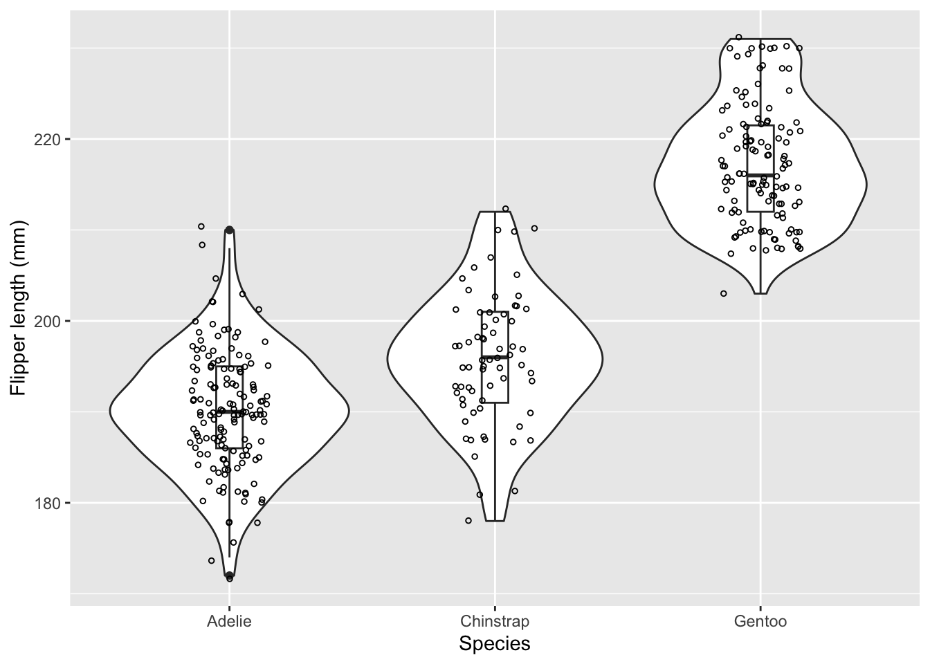
An ANOVA test with two groups is equivalent to a two-sample t-test. Unlike two-sample t-tests, ANOVA can simultaneously test many groups without inflating the Type I error rate beyond \(\alpha\).
Here is an example of using ANOVA to test whether the mean flipper length is different between three different species of penguins.
Since we have large sample sizes, it would be helpful to visualize the data with a violin plot (or a boxplot would work too).
palmerpenguins %>%
ggplot(aes(x = species, y = flipper_length_mm)) +
geom_violin() +
geom_boxplot(width = 0.1) +
geom_jitter(size = 1, shape = 1, width = 0.15) +
xlab('Species') +
ylab('Flipper length (mm)')
The null hypothesis for an ANOVA test is that the population means, \(\mu_i\), are the same for all treatments. The alternate hypothesis is that at least one population mean is different from the rest. ANOVA cannot give us information about which group’s population mean is different from the rest.
We’ll be conducting a fixed-effects ANOVA test, which uses the F-test statistic.
ANOVA makes the same assumptions as a two-sample t-test:
We can check the normality assumption using a normal quantile plot:
palmerpenguins %>%
  ggplot(aes(sample = flipper_length_mm)) +
  stat_qq(shape = 1) +
  stat_qq_line() +
  facet_grid(~ species) +
  xlab('Normal quantile') +
  ylab('Flipper length (mm)')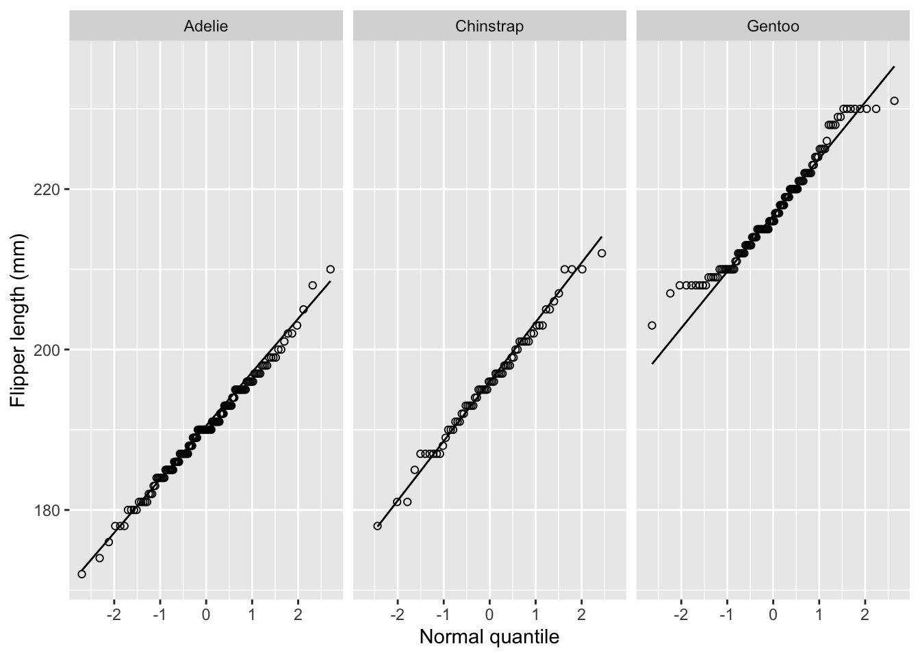
We can check the homoscedasticity (equal variances) assumption using the Bartlett’s test:
bartlett.test(flipper_length_mm ~ species, data = palmerpenguins)
    Bartlett test of homogeneity of variances

data:  flipper_length_mm by species
Bartlett's K-squared = 0.80702, df = 2, p-value = 0.668
Since the P-value is greater than 0.05, we fail to reject the null hypothesis of equal variances.
There are two steps to performing an ANOVA test in R. First, we need to create a linear model using the lm function. Then, we can pass that to the anova method to generate the appropriate ANOVA results.
palmerpenguins.lm <- lm(flipper_length_mm ~ species, data = palmerpenguins)
anova(palmerpenguins.lm)
Analysis of Variance Table
Response: flipper_length_mm
Df Sum Sq Mean Sq F value Pr(>F)
species 2 50526 25262.9 567.41 < 2.2e-16 ***
Residuals 330 14693 44.5
---
Signif. codes: 0 '***' 0.001 '**' 0.01 '*' 0.05 '.' 0.1 ' ' 1| \(df\) | Sum of Squares | Mean of Squares | \(F\)-ratio | \(P\) | |
|---|---|---|---|---|---|
| Species | 2 | 50526 | 25262.9 | 567.41 | 2.2e-16 |
| Residuals | 330 | 14693 | 44.5 |
Due to the low P-value, we can reject the null hypothesis that the mean flipper length is equal. But now the question is, which group mean(s) differ?
The Tukey-Kramer post-hoc test (yes, a mouthful) compares all group means to all other group means. This is preferable to doing multiple two-sample t-tests because the latter inflates the Type I error rate.
To conduct this test in R, we first need to re-do the ANOVA test using the aov method and pass that onto TukeyHSD(). An example is shown below:
aov(flipper_length_mm ~ species, data = palmerpenguins) %>%
  TukeyHSD(conf.level = 0.95)
Tukey multiple comparisons of means
95% family-wise confidence level
Fit: aov(formula = flipper_length_mm ~ species, data = palmerpenguins)
$species
diff lwr upr p adj
Chinstrap-Adelie 5.72079 3.414364 8.027215 0
Gentoo-Adelie 27.13255 25.192399 29.072709 0
Gentoo-Chinstrap 21.41176 19.023644 23.799885 0