anorexia <- anorexia %>%
  mutate(diff = Post - Prior, id = row_number()) %>%
  pivot_longer(c('Prior', 'Post'), names_to = 'time', values_to = 'weight')

anorexia$time <- ordered(anorexia$time, levels=c('Prior', 'Post'))4 Paired t-test
This is a test used to analyze the difference between the means of two treatments/groups where the samples are paired. The two treatments are applied to separate, independent samples.
We have a dataset with the weights of 17 girls before and after treatment for anorexia. Since the same individuals were measured twice, we can use a paired t-test to see if the treatment worked.
Before we start, we can store the differences in each pair as another variable and tidy the data, converting to long format. I’m also storing the row numbers as a column so that we know which before row corresponds to which after row, and ordering them such that Prior shows up before Post (as opposed to alphabetical order).
4.1 Visualizing data
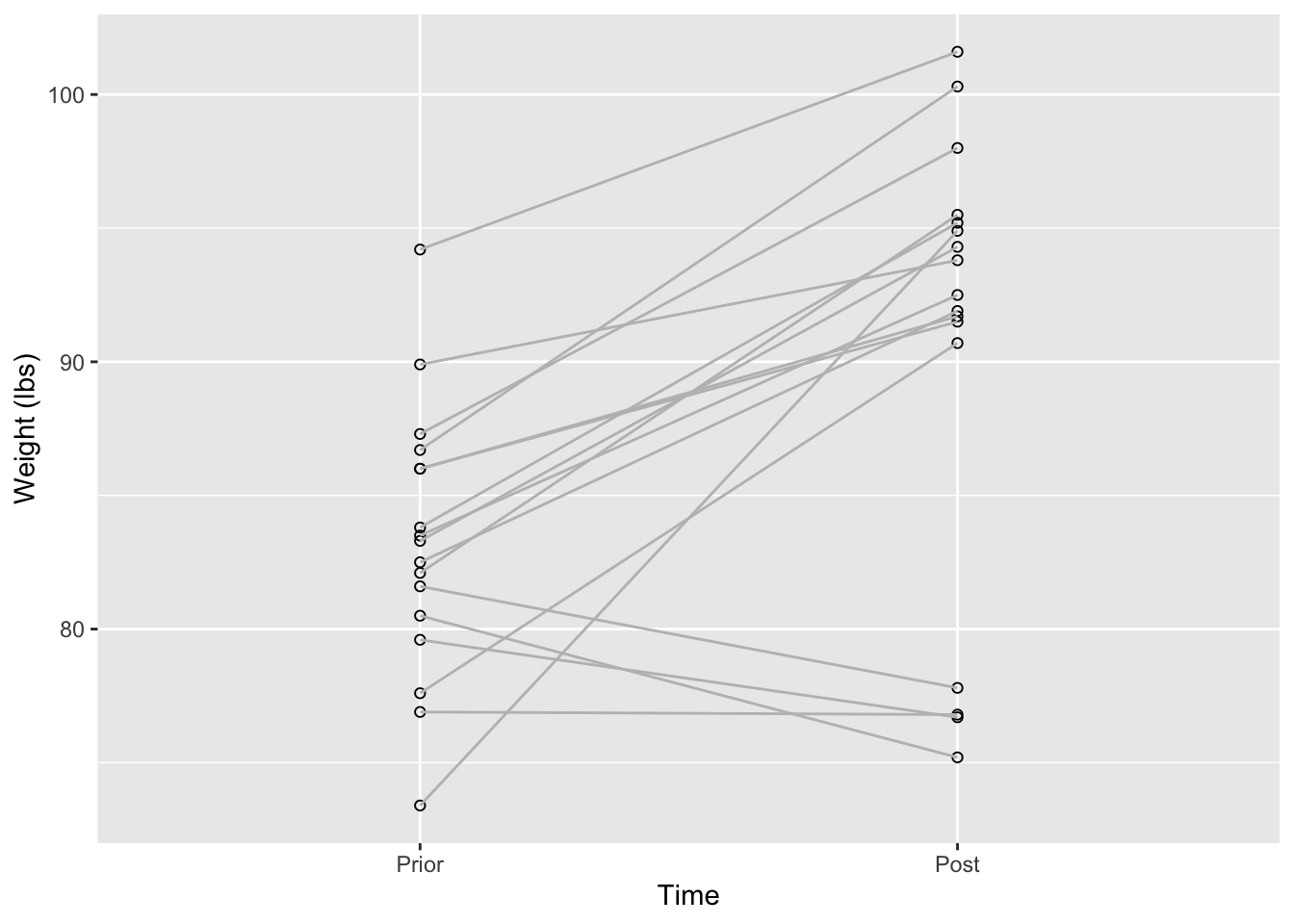
A typical way to visualize the differences for a paired t-test is using a plot like this.
anorexia %>%
  ggplot(aes(x = time, y = weight)) +
  geom_point(shape = 1) +
  geom_line(aes(group = id), color = 'grey') +
  xlab('Time') +
  ylab('Weight (lbs)')
4.2 Hypotheses
The hypothesis of a paired t-test is all about the mean of the difference in the pairs, \(\mu_d\):
- \(H_0\): The mean change in weight after anorexia treatment was 0.
- \(H_A\): The mean change in weight after anorexia treatment was not 0.
Or symbolically, it can be represented as:
- \(H_0: \mu_d = 0\)
- \(H_A: \mu_d \neq 0\)
4.3 Checking assumptions
The assumptions for conducting a paired t-test are as follows:
- The individuals are randomly sampled from the population.
- The differences are normally distributed in the population.
Since the sample size is so small, a normal quantile plot may not be as helpful in evaluating the normality of the data. Alternatively, it can be verified by conducting a Shapiro-Wilk normality test, which checks the null hypothesis that the data are sampled from a normal distribution:
shapiro.test(anorexia$diff)
    Shapiro-Wilk normality test

data:  anorexia$diff
W = 0.94074, p-value = 0.06484
Since the P-value is greater than 0.05, we fail to reject the \(H_0\) of normality and can proceed with the test.
4.4 Performing a paired t-test
We can use the built-in t.test method in R to perform this test. If you need help using this command, you can use ?t.test to view the documentation for this command.
t.test(weight ~ time, data = anorexia,
  paired = TRUE, conf.level = 0.95)
    Paired t-test

data:  weight by time
t = -4.1849, df = 16, p-value = 0.0007003
alternative hypothesis: true mean difference is not equal to 0
95 percent confidence interval:
 -10.94471  -3.58470
sample estimates:
mean difference
      -7.264706
Since the test produced a P-value less than 0.05 (\(\alpha\)), we can reject the null hypothesis.