beaver %>%
  ggplot(aes(x = activ, y = temp)) +
  geom_boxplot(width = 0.1) +
  xlab('Activity') +
  ylab('Body temperature (°C)')
This is a test used to analyze the difference between the means of two treatments/groups where the samples are not paired. The two treatments are applied to separate, independent samples.
Here is an example of how to conduct a two-sample t-test using a dataset on the body temperatures of active and inactive beavers.
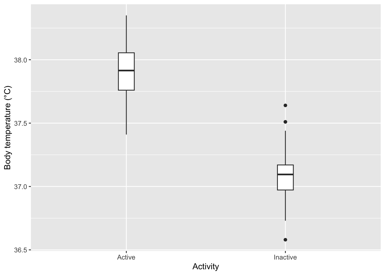
We could visualize our data using a boxplot since we’re trying to see the association between a categorical and a numerical value.
beaver %>%
ggplot(aes(x = activ, y = temp)) +
geom_boxplot(width = 0.1) +
xlab('Activity') +
ylab('Body temperature (°C)')
It seems likely that active beavers have a higher mean body temperature than inactive beavers, but we can verify this using the two-sample t-test.
We can state the hypotheses for the test as follows:
We can let \(\mu_1\) represent the mean body temperature of active beavers and \(\mu_2\) represent the mean body temperature of inactive beavers, and rewrite our hypotheses in symbolic format:
The first two assumptions of this test are the same as the two-sample t-test. The additional assumption is listed below.
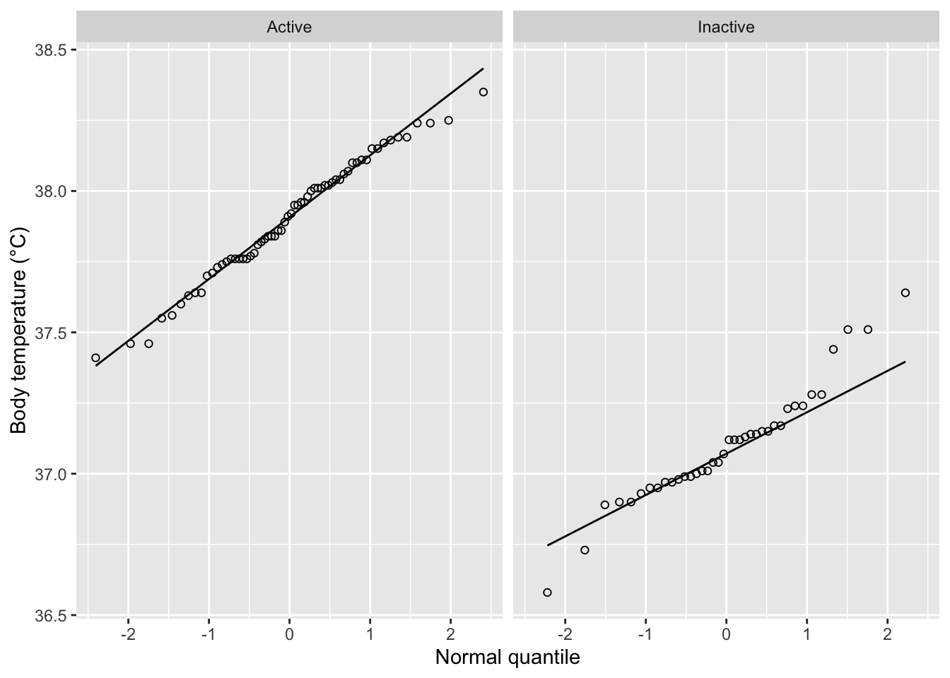
For our purposes, the normality assumption can be verified using a normal quantile plot:
beaver %>%
  ggplot(aes(sample=temp)) +
  stat_qq(shape = 1) +
  stat_qq_line() +
  facet_grid(~ activ) +
  xlab('Normal quantile') +
  ylab('Body temperature (°C)')
From the qq plot above, both groups seem to be drawn from normal populations. Next, we can also check the equal-variance assumption using the F-test:
var.test(temp ~ activ, data = beaver)
    F test to compare two variances

data:  temp by activ
F = 1.0841, num df = 61, denom df = 37, p-value = 0.8045
alternative hypothesis: true ratio of variances is not equal to 1
95 percent confidence interval:
 0.5912487 1.9053969
sample estimates:
ratio of variances
          1.084081
Since the P-value for the F-test is greater than 0.05, we fail to reject the null hypothesis of equal variance.
We can use the built-in t.test method in R to perform this test. If you need help using this command, you can use ?t.test to view the documentation for this command.
t.test(temp ~ activ, data = beaver,
  paired = FALSE, var.equal = TRUE, alternative = 'greater',
  conf.level = 0.95)
    Two Sample t-test

data:  temp by activ
t = 18.367, df = 98, p-value < 2.2e-16
alternative hypothesis: true difference in means between group Active and group Inactive is greater than 0
95 percent confidence interval:
 0.7333337       Inf
sample estimates:
  mean in group Active mean in group Inactive
              37.90306               37.09684
Since the test produced a P-value less than 0.05 (\(\alpha\)), we can reject the null hypothesis.